import pandas as pdimport numpy as npfrom sklearn.ensemble import RandomForestClassifierfrom sklearn.model_selection import train_test_splitfrom sklearn.datasets import fetch_openmlfrom sklearn.metrics import classification_report, precision_score, recall_score, f1_score, confusion_matriximport matplotlib.pyplot as pltfrom tqdm import tqdmimport psutil
Load data
X, y = fetch_openml('mnist_784', version=1, data_home='data', return_X_y=True, as_frame=False)
/home/patel_zeel/miniconda3/lib/python3.9/site-packages/sklearn/datasets/_openml.py:1002: FutureWarning: The default value of `parser` will change from `'liac-arff'` to `'auto'` in 1.4. You can set `parser='auto'` to silence this warning. Therefore, an `ImportError` will be raised from 1.4 if the dataset is dense and pandas is not installed. Note that the pandas parser may return different data types. See the Notes Section in fetch_openml's API doc for details.
  warn(
train_size =200X_train, X_pool, y_c_train, y_c_pool = train_test_split(X, y_c, train_size=train_size, random_state=42)print(X_train.shape, X_pool.shape, y_c_train.shape, y_c_pool.shape)# plot a bar chart of the number of samples in each class for the training and test setunique, counts = np.unique(y_c_train, return_counts=True)print("Number of samples in each class for training set", dict(zip(unique, counts)))print("One v/s rest ratio", counts[0]/counts[1], "for training set")
(200, 784) (69800, 784) (200,) (69800,)
Number of samples in each class for training set {0: 179, 1: 21}
One v/s rest ratio 8.523809523809524 for training set
Prof. Ermon’s method
X_train, X_pool, y_c_train, y_c_pool = train_test_split(X, y_c, train_size=train_size, random_state=42)print(X_train.shape, X_pool.shape, y_c_train.shape, y_c_pool.shape)clf = RandomForestClassifier(n_estimators=100, max_depth=10, random_state=0, n_jobs=psutil.cpu_count()//2)clf.fit(X_train, y_c_train)preds = clf.predict(X_test)test_recall = [recall_score(y_c_test, preds)]test_precision = [precision_score(y_c_test, preds)]positives = [np.sum(y_c_train)]negatives = [len(y_c_train) - positives[-1]]labeling_cost = [0]tp = np.where((preds ==1) & (y_c_test ==1))[0]fp = np.where((preds ==1) & (y_c_test ==0))[0]print("Test: Number of false positives", len(fp), "Number of true positives", len(tp))print("Iteration", 0, "Precision", test_precision[-1], "Recall", test_recall[-1], "Cost", labeling_cost[-1])al_iters =10foriterinrange(al_iters):print() preds = clf.predict(X_pool)# pred_proba = clf.predict_proba(X_pool)# print(pred_proba.shape)# identify instances predicted as positive but are actually negative (false positives)# we only pick points with more than 90% probability of being positive# fp = np.where((pred_proba[:, 1] > 0.8) & (y_pool == 0))[0] fp = np.where((preds ==1) & (y_c_pool ==0))[0] tp = np.where((preds ==1) & (y_c_pool ==1))[0] fn = np.where((preds ==0) & (y_c_pool ==1))[0]print("Pool: Number of false positives", len(fp), "Number of true positives", len(tp), "Number of false negatives", len(fn)) tp_fp = np.concatenate((tp, fp))# add them to the training set X_train = np.concatenate((X_train, X_pool[tp_fp])) y_c_train = np.concatenate((y_c_train, y_c_pool[tp_fp])) positives.append(np.sum(y_c_train)) negatives.append(len(y_c_train) - positives[-1])# remove from the pool set X_pool = np.delete(X_pool, tp_fp, axis=0) y_c_pool = np.delete(y_c_pool, tp_fp)# add the cost of labeling to the list labeling_cost.append(len(tp_fp))# train the classifier again clf.fit(X_train, y_c_train)# predict on the test set preds = clf.predict(X_test) tp = np.where((preds ==1) & (y_c_test ==1))[0] fp = np.where((preds ==1) & (y_c_test ==0))[0] fn = np.where((preds ==0) & (y_c_test ==1))[0]print("Test: Number of false positives", len(fp), "Number of true positives", len(tp), "Number of false negatives", len(fn))# calculate precision and recall test_recall.append(recall_score(y_c_test, preds)) test_precision.append(precision_score(y_c_test, preds))# print informationprint("Iteration", iter+1, "Precision", test_precision[-1], "Recall", test_recall[-1], "Cost", labeling_cost[-1])labeling_cost = np.cumsum(labeling_cost)
(200, 784) (69800, 784) (200,) (69800,)
Test: Number of false positives 8 Number of true positives 283
Iteration 0 Precision 0.9725085910652921 Recall 0.2742248062015504 Cost 0
Pool: Number of false positives 73 Number of true positives 1884 Number of false negatives 5085
Test: Number of false positives 209 Number of true positives 932 Number of false negatives 100
Iteration 1 Precision 0.8168273444347064 Recall 0.9031007751937985 Cost 1957
Pool: Number of false positives 1389 Number of true positives 4386 Number of false negatives 699
Test: Number of false positives 489 Number of true positives 1016 Number of false negatives 16
Iteration 2 Precision 0.6750830564784053 Recall 0.9844961240310077 Cost 5775
Pool: Number of false positives 4088 Number of true positives 598 Number of false negatives 101
Test: Number of false positives 12 Number of true positives 1006 Number of false negatives 26
Iteration 3 Precision 0.9882121807465619 Recall 0.9748062015503876 Cost 4686
Pool: Number of false positives 18 Number of true positives 15 Number of false negatives 86
Test: Number of false positives 10 Number of true positives 1010 Number of false negatives 22
Iteration 4 Precision 0.9901960784313726 Recall 0.9786821705426356 Cost 33
Pool: Number of false positives 13 Number of true positives 5 Number of false negatives 81
Test: Number of false positives 11 Number of true positives 1010 Number of false negatives 22
Iteration 5 Precision 0.9892262487757101 Recall 0.9786821705426356 Cost 18
Pool: Number of false positives 5 Number of true positives 2 Number of false negatives 79
Test: Number of false positives 10 Number of true positives 1011 Number of false negatives 21
Iteration 6 Precision 0.990205680705191 Recall 0.9796511627906976 Cost 7
Pool: Number of false positives 5 Number of true positives 1 Number of false negatives 78
Test: Number of false positives 9 Number of true positives 1011 Number of false negatives 21
Iteration 7 Precision 0.9911764705882353 Recall 0.9796511627906976 Cost 6
Pool: Number of false positives 5 Number of true positives 2 Number of false negatives 76
Test: Number of false positives 11 Number of true positives 1010 Number of false negatives 22
Iteration 8 Precision 0.9892262487757101 Recall 0.9786821705426356 Cost 7
Pool: Number of false positives 5 Number of true positives 2 Number of false negatives 74
Test: Number of false positives 9 Number of true positives 1010 Number of false negatives 22
Iteration 9 Precision 0.9911678115799804 Recall 0.9786821705426356 Cost 7
Pool: Number of false positives 3 Number of true positives 1 Number of false negatives 73
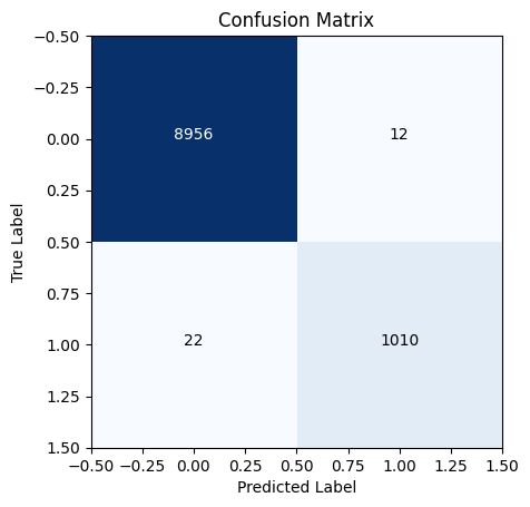
Test: Number of false positives 12 Number of true positives 1010 Number of false negatives 22
Iteration 10 Precision 0.9882583170254403 Recall 0.9786821705426356 Cost 4
# plot the confusion matriximport itertoolscm = confusion_matrix(y_c_test, preds)plt.imshow(cm, interpolation="nearest", cmap=plt.cm.Blues)# add the numbers inside the boxesthresh = cm.max() /2.0for i, j in itertools.product(range(cm.shape[0]), range(cm.shape[1])): plt.text(j, i, cm[i, j], horizontalalignment="center", color="white"if cm[i, j] > thresh else"black")plt.title("Confusion Matrix")plt.xlabel("Predicted Label")plt.ylabel("True Label")